VOLATILITY

No one has missed the tremendous rise in volatility in september and even more in oktober: the VIX index thee-doubled in the value since the beginning of september. We saw intraday movements only normally seen in months. It is also the sudden change in volatility that has surprised many people.

Look at the VIX data at the yahoo website during the last 6 months and for a comparison a chart since 1990. It seems that all of a sudden the world has completely changed since oktober. In reality it hasnot.






(Data from Yahoo)

Quite a while ago I wrote an article about intrady movements on the German Future DAX in a magazine called Traders.

There I defined volatility as the difference between the daily Highs minus the daily Lows because this value being really of importance for daytraders as they feel this movement throughout the day.

The data were gathered and various statistical tests were performed with it. One of the aims was to see if the data would fit in some distribution. It was no surprise that these data did not fit in a normal ditribution. It is almost ridiculous now to think of normality data returns.

The best guess then was the General Extreme Value distribution (GEV). These kind of distributions are known from Extreme Value Theories, fairly complicated material and for more details I refer to my article.

Some of the conclussions drawn from the article were:
Importantly the intraday movements do not follow a normal distribution but exhibit a fat right tail and skewness to the right. The non normality of these intraday movements has consequences for risk analysis (.. as done in VaR calculations).

The observation of bigger intraday movements than could be expected when normally distributed has consequences for risk management. Fitting data in a Fisher-Tippett or GEV distribution and looking at the relevant cumulative distribution gives a much better insight in the possible intraday movements of the FDAX and thus in the risk you may expect, but also in the opportunities this gives.

This was a good thought and seems to be totally right (but not followed by the so called professionals).

PREDICTION OF THE FUTURE IN TRADING

It is a general knowledge that the future cannot be predicted. Nobody knows exactly what will happen tomorrow let alone in a year. This fact leaves us with a very uncertain feelings and no surprise that a deep drive to try to control the environment and the future.

This can be seen in almost every field where humans operate: from production processes in factories to climate change models. Also traders face the challenge of dealing with the future.

Various methods exist to control and to get grip on the future and all of them are used by traders. Indicators, chart patterns, the use of regular cycles in one or other way (Gann), astrology and so on.

A good starting point to value these methods is to understand that future prices of assets cannot be predicted in general and the only way to deal with this is to use a concept of expectation of the future. An example with throwing a dice naturally comes in mind here.

Everyone knows that throwing a fair dice enough times will result in equally divided amount of the faces coming up. This is the same as saying the probability of a one, a two etc. is exactly 1/6. Our expectation of throwing a fair dice is 1/6 and so we know the future of this dice throwing process fairly well.

There is only one key assumption made here: a dice has to be a fair one. This is crucial. The consequence of using a fair dice is that it can be shown in a mathematical way that the expectation of throwing a fair dice is 1/6. This concept is used in our daily lives over and over again and used by traders. But here is also a big bootstrap.

Mathematics is not physics. Though the assumption of a fair dice maybe in reality a fairly good one (in fact, the contrary is assumed, if throwing a dice is not coming with our expectation of it, we assume the dice to be not fair). We are never sure if a dice is a perfect dice in a way that no imperfections exist with its faces which would result in unexpected results. Even when we know that such small imperfections exist we also know that it may not lead to in a different outcome when throwing it.

The understanding of this has consequences for our daily lives and the understanding of our evolution as human and so philosophical implications too.

Two examples from Traders of February may clarify my thoughts about this. The first one is about a so called Delta phenomenon from Marko Graenitz and the second from Tomasini and Jaecle about the use of indicators.

The Delta phenomenon is proposed to predict the future moves of commodities. The author shows how this delta is performing when used for the FDAX and the FTSE. It shows a fairly good forecast at the end of 2005 to 31 December 2006 for both of them compared with the actual chart. Without going into the question how good these predictions are (goodness of fit), two remarks have to be made here.

The apparent good prediction for these two index futures does not necessarily mean much if you realize that these are made over the same period of time because many if not all index futures showed the same strong upward movement the last year and the Delta would produce the same result for all of these indices used over the same time span.

The second critical remark is the following: whenever a prediction is made about the future that afterwards proved to be accurate what does this say about other predictions over other timeframes in other circumstances? When something seems to work here, does it still work there and there and then?

Think about the predictions of soccer games on Saturday or Sunday: there will be once in while someone who predicts all twelve games correctly, as there will always be somebody who predicted in the past the current oil price and so on. In the same line, always something can be found that predicts at a certain time fairly good a price in the future.

Another example is proposed by Tomasini and Jaekle. They propose a system based on a short period indicator and a filter of a longer period to obtain trade entries. The result is a very promising equity curve based on serious performed back tests over more than 600 trade entries during 3 years.

The question is off course, does the system produce the same results in the future.
This question is basically this: are results from a certain period in the past significant for a bigger period, a period also including the future in terms of expectation? In a way this can be stated as follows: is finding a good back testing result the same as finding a fair dice?

What I missed in these tests is at least a so called out of date test (sometimes referred as a forward test), a simulation of the system in real time. It will not be the first a time a good back testing does not result in good forward testing which is sometimes partly due to wrong interpretations of the back testing or partly to other factors. Also and very important the period which was tested may just not to be significant for the overall performances o the system.

CONSEQUTIVE LOSSES

In two lucid and interesting articles in Traders of January two subjects were discussed, subjects I studied extensively. Luca Barberis tried to give an answer to the question how trading of various markets can enhance the equity curve without optimising individual trading systems. Optimising hides the danger of curve fitting. Though his results are very important a few aspects remains to be answered before applying his method: how many contracts do you trade the various markets, which is not a matter of classical position sizing matters and the question of a possible trade system correlation and what effect this has on risk.

Risk is the main subject of Philip Kahler in Traders. He treats various possible types of risk in trading, especially risk due to consecutive losses and emphasizes its importance to understand how consecutive losses can influence trading results. When studying consecutive losses in series of trades a huge field opens up: many different theoretical frameworks can be set up to master this phenomenon of trading.

There is a clear relation between the win ratio of a trade system and the length of consecutive losses. In an earlier post I stressed the importance of the win ratio in a different context. But it also plays an important role in the existence, the length, and the amount of consecutive losses.

In general can be said that the higher the win ratio the higher the chance becomes for a series of losses of a certain length. In his article Kahler gives some examples and a graphic which can be used to determine 5 or 10 consecutive losses for a given win ratio. It has to be said that these probabilities occur for a given amount of trades performed and will change negatively when the total trades increases.

Though interesting to know the chance for a series of losses it would be even more interesting to know a distribution of series of losses, e.g. the probability for all possible series of losses and moreover the maximum length of consecutive losses (maximum streak) you might expect for a given win ratio.

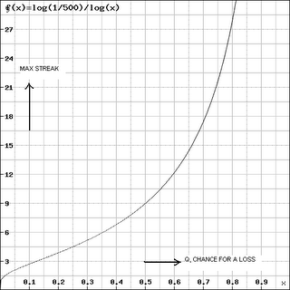
Below you can see a figure which gives the relation for the maximum streak and the probability of a loss (loss ratio). Total trades is 500, confidence is 0.998%.




From this figure again can be seen the importance of the loss ratio: the higher this becomes (the more losses)then the maximum strak increases exponentially. E.g when q, the probability of a loss is 35% then the maximum expected streak willl be 6 but when increasing to 70% the maximum streak increases to 17 consequtive losses in a row!

LUCK AND CHANGE ON THE MARKET

My partner and I spent the week around Christmas in Mumbai, India. Mumbai is the financial and economic centre of India. The Bombay Stock Exchange (BSE) had a splendid year behind with a year output of more than 33%.

From local newspapers a moderate hosanna mood can be felt. Also internationally India got much attention in the last year. It is particularly the growing middle class that forms the driving force behind the economy and which gets attention of foreign investors.

With an increase of 33% the BSE is one of the best performing markets in the world. Of course it must immediately be said that almost all markets performed very well. The phenomenon that markets are moving more or less in the same direction is called correlation.

Correlation between markets is high: data which I have collected on 15 minutes basis of the futures on the FDAX and the DOW JONES appear to have a correlation of more than 90% over the past 2 years. This is almost complete correlation.

Now the question arises if a result such as that of the Bombay Stock Exchange can be attributed to well performing of the Indian economy or that also chance may play a role in it. It cannot be denied that chance and luck play an important role on the markets.

Let’s have a look at this without going into this matter to deeply. Suppose that an invisible hand would assign the different markets worldwide a return around a certain average. Then you may expect these returns to be divided normally.

A quick lookup at the financial site of Yahoo reveals the following. Of the 17 most important markets there is not one with a negative output over 2006. The output diverges from 10% (London) up to 55% (Moscow) with an average of rounded 24%. The spread, standard deviation amounts to 23%. This means that if the 17 markets are representative for all markets in the world, about 66% of all markets will show an output of 1 standard deviation above or below the average (therefore 24% ± 23%). Of all 17 markets there are only 2 outside this range.

We can look at this also in a different way: we can consider the return of an individual market as an estimate of the world average and look at how well such an estimate would be.

It is known that such an estimate will have a standard error that equals to σ/√T where σ is the annual volatility and T the number of years:

STD = σ/√T (1)


From formula (1) it follows that the standard error of an estimate of the world average decreases with the square root of the number of years.

Let’s take Mumbai as an example. The excess return or α, of this market above the world average is 33-24 = 9%. Though in general the term α refers to the excess return of a fund with respect to the benchmark, it may also be used for the excess return of a market.

To be convinced that an excess return is the consequence of a better performing of the economy and not to pure chance or luck then the return must be bigger than the world average with a significant size. In a one-sided test at the 95% confidence level the difference between the two must be greater than 1.65 standard deviations.

Suppose the volatility to be around 20% on an annual basis for the Bombay market then the standard error according to (1) will be 20%/√1 = 20%. The 9% above the average of the market is clearly smaller than one standard deviation above the average, clearly below 95% confidence level. It lies approximately at 50% what means that 50% of the return of Bombay falls to pure chance. In fact you can say that the 33% return of Mumbai is a good estimate of the world average.

We can carry out this calculation also differently and perhaps it will even become more clearly then. We saw that the standard error of an estimate of the average decreases with the square root of the number of years taken into account.

We know that: α =9% = 1,65* STD. It follows that STD, the standard error, equals 9/1,65 = 5,45. This value substituted for the STD in formula (1) gives √T = 23% /5,45 = 4.22 ==> T = 17,8 year.

This means therefore that the Bombay Stock Exchange for at least 17 years in succession must show a return that 9% or more lies above the world average to be able to say that for 95% this is due to a better performing of the economy and only for 5% to chance.

Around these days various funds present their performances. Some will show better results than others. From the previous it must be clear that luck may play a large role besides skill of the fund managers and in any case is much larger than they will admit. Think to that.

CONSISTENCY AND SHARPE RATIO (1)

For me consistency has always been a very important and interesting factor in trading. By consistency I mean how long, in a given timeframe, let say 12 months or 12 weeks, my trades are giving a positive result. Can I expect 6 months out of 12 being profitable or more or less? This is one of the questions which I always try to give as best as possible an answer.

One of the most used criteria for evaluating fund managers is the Sharpe Ratio. The Sharpe Ratio is used for this because of its easy use: the bigger the Sharpe the better the fund or the fund manager. This almost has become fait accompli.

How is the Sharpe Ratio calculated? It is simple obtained by dividing the average net profit (mean or expectation E) by the standard deviation of the trades. The standard deviation is, as you may know, a measure for the spread of winners of losers around the mean. Because the deviation is a measure for the trade spread it is also considered as a measure for the risk of the fund or the fund manager, but this standard deviation is also defined as the volatility of the fund.

The Sharpe ratio is in this way defined as the mean profit of the fund (-manager) per point risk or volatility. The bigger the mean, the bigger the Sharpe the better the fund (-manager) is performing. That's the idea.

An example. Suppose trader A has a gain of 5 ES points per trade, a spread of 10 points, done over 100 trades in one year. This means that, when trader's A profits are normally distributed over the losses and the winners, 99,73% of his trade outcomes is lying between 5 minus 30 (=-20) and 5+ 30 (=35). The Sharpe ratio is now 5/10 = 0.5 .

Do you see how it works? When the trade outcomes would have a bigger spread but with the same mean the Sharpe ratio would decrease, the mean per point risk will decrease.

When you look closely at the Sharpe Ratio you will see and understand that is in fact a measure for consistency. To see this take the next example. Trader B takes 100 trades a year but with every trade being a winner (if this would be possible, but for clarity reasons taken here) for 5 points. His net profitability and mean is the same as for trader A but his Sharpe ratio becomes 5/∞ = ∞. His consistency is 100%.

We defined the Sharpe ratio as the mean defined by the spread. This is not precisely correct. The exact definition is the excess profit over a zero risk profit divided by the spread. A zero risk is generally the return of a 30 year T-bond but also a European long bond could be taken. Off course the risk is not exactly zero but is considered to be and also T- bond returns are changing over time (inflation).

Our definition of the Sharpe is a modified Sharpe, but it doesn't really matter, because the exact definition doesn't give more information. You only have bear in mind how the Sharpe is defined when it is used in comparisons.

There is a clear relation with so called z score of a normal distribution and a lookup in a table with a z 0f ∞ gives a 100% consistency. In this way consistency can be defined and I use it this way.

But before closing this post three remarks have to be made.

1. The Sharpe and the consistency is defined for normal distributed trade returns but in practice returns seldom are.

2. The spread as a measure is not a very good one because in this way it also takes positive returns as a risk and this is not what traders and investors generally feel about positive returns.

3. The longer a trader stays in business the bigger his draw downs will be. Or said otherwise: the more trades a fund manager takes the bigger his draw downs will be, or said it in another way: the more trades a fund manager takes, how bigger his drawdown. The consequence is that the longer a fund manager is in business (the longer a fund exists) he will be punished with a lowering of his Sharpe ratio. I will come back to this in my next post.

So the conclusion is that Sharpe is a useful concept but not more and so other concepts for consistency are needed. These are the Sortino Ratio, Callmar ratio and the Martin Ratio. I developed another concept of consistency which I called Excess Loss Wealth Function (ELWF) which I draw directly from the theory of random walks.

TRADE SYSTEMS AS SUCH

Last time I was talking about expectations and the use of stops. One of the things that interested me was the relation between a stop and other system parameters like amount of losses/winners and the average win/loss. I stated that for a given trade system a clear relation between these parameters doesn't exist.

But, as you may have noticed in earlier postings I wrote about the win ratio and it's relation to expectation. I described expectation in terms of win ratio (chance of a winner) and one of the things I found was a clear relation between the win ratio and the profit ratio (= average/average loss. From the figure given there some conclusions cold be drawn how big the profit ratio has to be with a given win ratio for the expectancy to be positive.

Now, you could ask, is this in contradiction with findings in my last post?. It is maybe a surprise but I think there isn't.

When I tried to describe a relation between expectancy and win ratio I was primarily interested to let you see the importance of a high win ratio, in contrary to some, or most, writers who stress the importance of an overall profit but ignore to tell you the serious problems you encounter when your trading systems comes up with only a few winners and a bunch of losers. They may be right but is it workable, see my last posting about expectancy and win ratio

So, in these postings I was comparingdifferent trade systems to each other. I then focussed one a particular system and its parameters. I have a strong conviction in the existence of trade systems as such, whose trade parameters are fixed. I think of trade systems as being some entity that produces so and so many trades a year, with a certain expectation per trade and profit factor. Seeing systems this way it is no longer a contradiction to say that parameters of a system in particular are dependant.

Now, the question is now as follows. When I or you try to trade this system, do we get the same results as theoretically would be possible? I already posted before about this (Luck and Randomness) and I suspected then some interesting aspects of trading on which I want to post in the future.

STOPS AND TRADING SYSTEMS

It is common to use stops to avoid big losses and to avoid the psychological danger a trader can have when he is uncertain to close his positions at time.

Still sometimes no stop is proposed in trading. We all now that too small a stop the will punch out too often, sometimes leaving us behind with a potential winner while too big a stop can have a big influence on our overall results.

Suppose someone trades 100 times a year of which 80% are small winners and mall losers. This is not an unreal situation for a discretionary trader. His results are determined by the last 20% which we suppose to be big winners and big losers.

The influence of one of such a trade is substantial. A big loser or big winner can make a substantial difference to the final results of the trader.
But the question remains if how losers and winners effect each ohter.

We know the concept of Expectancy:

E = P / NP - L / NL = Average Win – Average Loss (1)

In words: The expectation of a trade is the total win divided by the total amount of losses minus the total loss divided by the total amount of losers.

The above formula has four variables, P the total win, L, the total loss, NP the amount of winners and NL the amount of losers. Each of them can be changed, e.g. decreasing the the total loss L, decreases the average loss and so increases the sum which is the expectation E.

But changing one variable in formula (1), changing one may affect the other ones. The variables are said to be dependant from each other. For a given system, changing the average loss may result in changing the average win too!

An example: a system produces 100 trades a year, 60 losers and 40 winners. When 5 potential losses could eventually turned into 5 winners by taking a bigger stop the average win will increase due to this, but you may also expect that the average loss will increase due to the bigger stop of the remaining 35 losses. We also could go for bigger winners just to see an increase in the amount of losses.

We don’t know at forehand what happens and the problem stays. Suppose there is a function G with parameters NP, NL, P, L so that :

G (NP,NL,P,L).

G produces some results in terms of expectation E:

G (NP,NL,P,L) = f (E) (2)

I did some effort to investigate some general characteristics of formula (2). Though not being very being successfully it helped me I a better understanding the concept of a trading system, in fact a way of producing losers and winners which outcomes are dependant to each other.

One of the strangest things I found was that the outcome of a system is changing over time and not seldom worsening, not necessarily in terms of expectation E or E per dollar risk but more in terms of other characteristics as drawdown, amount of losses and winners, runs of losses and winners and so on.

This is a fundamental (stochastic) principle everywhere probability plays such an important role.